
Introduction
An estimated 80% of all organizational data is unstructured text. Despite this, even among data savvy organizations, most of it goes completely ignored. Why?
Numeric data is easy. Just toss it in a standard scaler, throw it at a model, and see what happens. You may not get good results, but you’ll get something, and you can always iterate from there.
Text data is hard. Before it can be entered into any mathematical model, it must first be encoded into numbers. How do we turn words into numbers? From simple 0’s and 1’s, to multidimensional embeddings, NLP has made incredible progress in the past decade. But using these cutting-edge strategies means rethinking our data. It means expanding our minds into complex higher-dimensional spaces that often defy our intuition.
I still struggle with the basic 4 dimensions of our physical world. When I first heard about 768-dimension embeddings, I feared my brain would escape from my ear. If you can relate, if you want to truly master the tricky subject of NLP encoding, this article is for you.
This is a deep dive: over 8,000 words long. Don’t be afraid to bookmark this article and read it in pieces. There is a lot to cover. We will start with basic One-Hot encoding, move on to word2vec word and sentence embeddings, build our own custom embeddings using R, and finally, work with the cutting-edge BERT model and its contextual embeddings.
Like Frodo on the way to Mordor, we have a long and challenging journey before us. Let’s get started.
Our Experiment
The “Lord of the Rings” and “Star Wars” are two iconic franchises that need no introduction. Every day thousands of passionate fans discuss these fictional worlds and characters online. For example:
Not quite. Radagast alerts the Eagles to scout around and report to him and to Gandalf. Gwaihir is near Orthanc later and sees Gandalf and so goes down to him. Radagast is not aware of Saruman’s Treachery at any point.
The above comment doesn’t specifically mention “Lord of the Rings”, but we humans can easily infer which franchise the author is talking about. Another example:
“For over a thousand generations the Jedi knights were the guardians of peace and justice in the old republic. Before the dark times. Before the empire.”- Ben Kenobi to Luke Skywalker.
Again, no specific mention of “Star Wars”, but we humans know what’s up. We can easily classify these comments. And in this experiment, we are going to train a machine to do the same thing.
Can different encoding methods help the machine gain better insights into the text? Do some methods result in better predictions than others? How do these different encoding methods compare, all else being equal?
Meet the Model
Our classifier is based on the StepByStep class by Daniel Voigt Godoy. It is an extremely simple model:
#define our model
model = nn.Sequential(
    nn.Linear(X, 1)
)
loss_fn = nn.BCEWithLogitsLoss()
optimizer = optim.Adam(model.parameters(), lr=0.01)

# train it
our_model = StepByStep(model, loss_fn, optimizer)
our_model.set_loaders(train_loader, val_loader)
our_model.train(100)
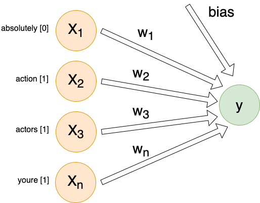
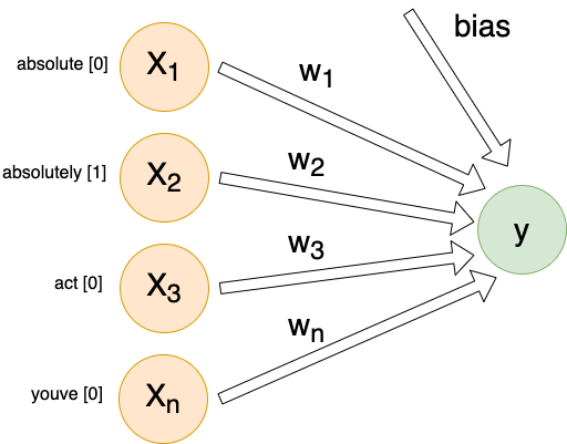
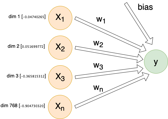
For each individual comment, we will send X inputs (features) into a dense linear layer with a single output. The exact number of inputs will differ depending on encoding method, but they will all follow this same architecture:
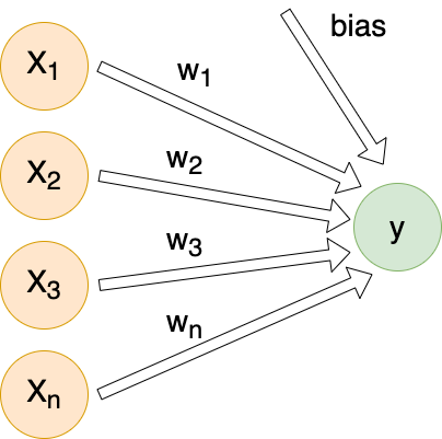
Each input (Xn) is connected to our output by its own weight (Wn). These weights, plus a special bias weight, are the trainable parameters of the model. We begin with random values. With each iteration these parameters (weights) are modified slightly.
This is what is happening behind-the-scenes when we say a model is training and learning. Mathematically speaking, we simply adjust each weight by the partial derivative of our loss function with respect to the given weight, multiplied by our learning rate (η).
![\[w_n\prime=w_n - \eta\frac{\partial \text{loss function}}{\partial w_n}\]](https://datajenius.com/wp-content/ql-cache/quicklatex.com-64c9f12d3934df330402b5c20d9b1704_l3.png "Rendered by QuickLaTeX.com")
Our model uses the Adam optimizer which adjusts our learning rate (η) as it trains. We will use the initial learning rate 0.01. In general practice, that learning rate is really big; we would normally use something closer to 0.0003.
That just leaves our loss function, the heart of any neural network. Since this is a binary classification task, we will use log loss. In general terms, this loss function measures the probability of belonging to the positive class . In our specific case we use BCEWithLogitsLoss which returns logits that must be passed through a sigmoid function to “squish” them back into these probabilities.
![\[S(x) = \frac{1}{1+e^{-x}}\]](https://datajenius.com/wp-content/ql-cache/quicklatex.com-a39bebbe262c2d0c19b8aee2c847d446_l3.png "Rendered by QuickLaTeX.com")
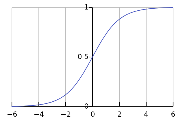
For any comments with a probability > 50%, we will classify them as positive. Here we treat “Lord of the Rings” as our positive class, but that is an arbitrary choice. The math works the same either way.
Same model, same data, different encoding methods. Here we go.
Our Data
On Reddit we find the /r/StarWars and /r/lotr subreddits. We wrote a simple reddit scraper using praw (google colab) to pull comments from each. We pulled about 50,000 comments total, from the “hottest” content around March 1, 2022.
A significant number of these comments were extremely short. They did not contain any useful information. Neither a human nor machine could tell you which subreddit they came from. We randomly selected 10,000 of these 50,000 total comments, each containing at least 13 words (not counting stop words e.g. “the”, “is”, “a”, etc.).
Exactly half of these comments came from /r/StarWars, and the other half from /r/lotr. This allows us to avoid the notorious imbalanced classes issue. If we used a coin flip to guess, or always picked the same franchise, we would expect to be right 50% of the time.

We used this R script to label and organize the data and break it into 5 equally sized 50/50 groups so we could put this data on github.
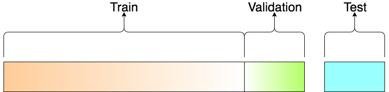
When training and testing models, we always want to remain mindful of data leakage. We cannot allow any information from outside the training dataset to “leak” into the model. To that end, we will use groups 1, 2 and 3 as our training data (60%), use group 4 as our validation data (20%), and leave group 5 as our testing data (20%).
This also helps keep everything as apples-to-apples as possible. Each method will be encoded, trained, validated and tested using the exact same samples.
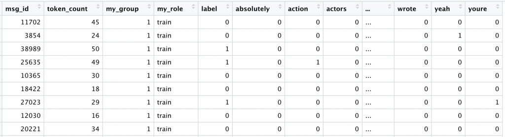
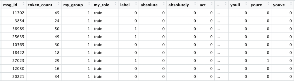
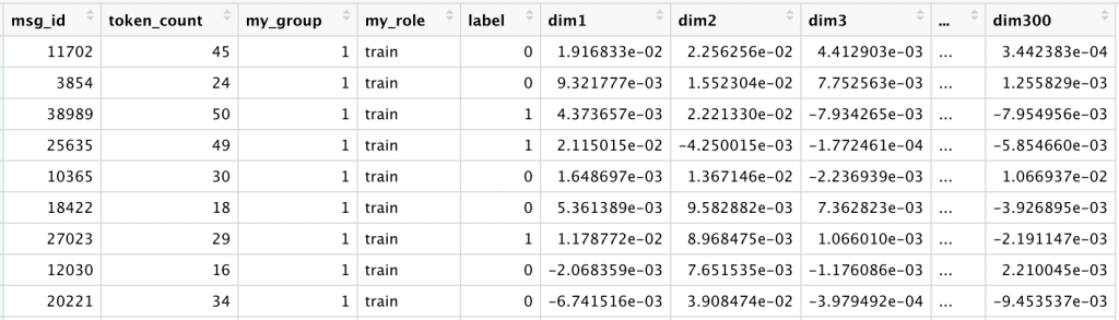
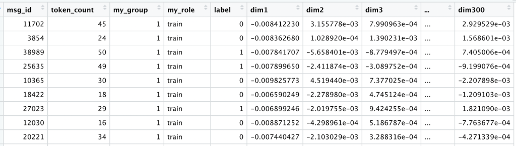
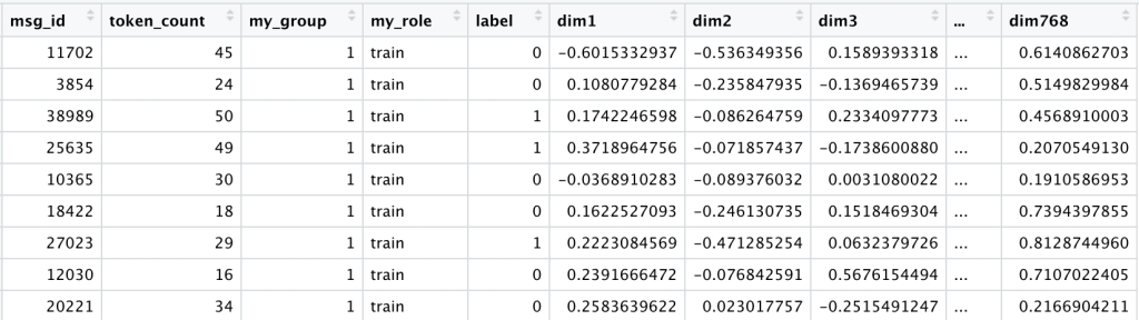
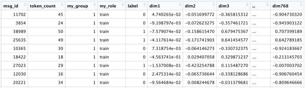
At this point our data looks like this:
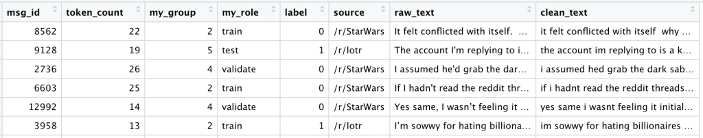
We keep the original raw_text exactly as written, plus a clean_text version, converted to lowercase, with all punctuation and other special characters removed.
Now how do we turn this data into input for our model?
One-Hot Encoding
We will begin with One-Hot encoded inputs. This will allow us to gain some insight into what our model is doing, and define some metrics for our model’s performance. This will also allow us to clearly illustrate the difference between tokenization and encoding.
Tokenizing with Unigrams
Tokenization is the process of turning a full text string into smaller chunks we call tokens. There are many different ways we might tokenize our text. We could use bigrams (“luke skywalker”) or trigrams (“gandalf the grey”), or tokenize parts of a word, or even individual characters. Our options seem infinite.
Here we will tokenize into unigrams, using the tidytext package in R. To avoid data leakage we will use only our training data here.
############################################
# load dependencies
library(tidyverse)
library(tidytext)

############################################################
# load our TRAINING data from github (groups 1, 2, 3)
comments <- read.csv("https://raw.githubusercontent.com/DataJenius/NLPEncodingExperiment/main/data/comments/selected/selected_reddit_comments_group1.csv") %>%
  rbind(read.csv("https://raw.githubusercontent.com/DataJenius/NLPEncodingExperiment/main/data/comments/selected/selected_reddit_comments_group2.csv")) %>%
  rbind(read.csv("https://raw.githubusercontent.com/DataJenius/NLPEncodingExperiment/main/data/comments/selected/selected_reddit_comments_group3.csv"))
We will tokenize on clean_text and also filter out any tokens that are stop words (common words such as “the” and “is” and “a”).
############################################################
# define our stopwords and make unigrams from clean_text
words_to_ignore <- stop_words$word
unigrams <- comments %>%
  unnest_tokens(token, clean_text) %>%
  filter(!(token %in% words_to_ignore))
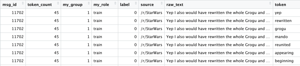
Even after filtering, we are left with a very long dataframe, with one row for each occurrence of each token:
Which of these tokens do we care about? How many documents (comments) does each token appear in?
################################################################
# find most important tokens according to document frequency
tokens_by_df <- unigrams %>%
  group_by(token) %>%
  summarise(total_df=length(unique(msg_id))) %>%
  arrange(desc(total_df))
Here is a list of the top 20 tokens by document frequency (df):
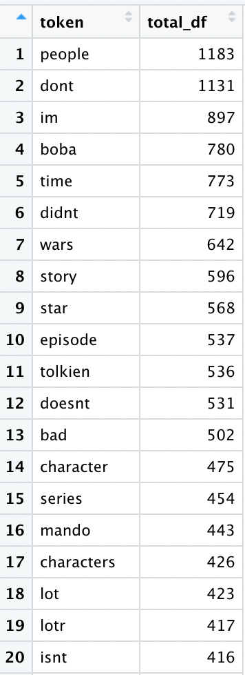
Some of our most frequent tokens (e.g. “story”, “tolkien”, “episode”) seem to offer insight into these two groups. Let’s visualize this:
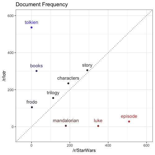
We see that some tokens (e.g. “trilogy”, “characters”, “story”) are used roughly the same by both franchises. Some tokens (e.g. “frodo”, “books”, “tolkien”) are used more often in /r/lotr comments, and others (e.g. “mandalorian”, “luke”, “episode”) are used more often in /r/StarWars comments.
But how do we get this information to our classification model?
Binary Encoding
One-Hot encoding is simple. If a comment includes a given token, we will mark that with a 1. If a comment does not include a given token, we will mark that with a 0. The only tricky part is deciding how many tokens to include. How much dimensionality do we want?
We begin with our top 300 tokens according to the document frequency of the training data. We then use that vocabulary to encode all 10,000 comments. At this point our data looks like this:
We have added a column for each of our top 300 tokens (starting with “absolutely”, “action”, “actors” and ending with “youre”). For each comment, if it includes a given token we see a 1, otherwise a 0. We can see this One-Hot encoding results in a sparse matrix; most of what it contains are 0’s.
You can find the R script used to one-hot encode the data, and the data itself on github. We started with a raw text string, tokenized it into clean tokens, and encoded these tokens into actual numbers (0 or 1) that can be passed into a neural network as input.
Limitations of One-Hot Encoding
Consider the following made up comments:
I love Luke Skywalker, but I hate Gandalf the Grey.
I love Gandalf the Grey, but I hate Luke Skywalker.
As humans we can see these two examples have opposite meanings. Sadly, our One-Hot encodings do not show any difference:
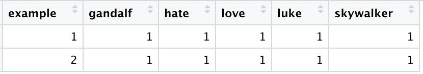
The order of tokens is ignored. Furthermore, only tokens that appear in our pre-defined vocabulary will appear here. Stop words like “I”, “the”, “but”, and less common tokens like “Grey”, simply disappear. We find 38 of these 10,000 comments are One-Hot encoded with all 0’s; they don’t contain any of the top 300 tokens.
Another issue: we only match exact tokens. For the sake of this encoding, “love” and “loved” are two entirely different things, even though, as humans, we understand they are just different forms of the same word. We also ignore how often these tokens are used.
How will our model do given these limitations?
One-Hot (300)
To train and use the model we turn back to python (google colab).
We will pass the model 300 inputs, 0’s or 1’s, for each of our top 300 tokens. This results in 301 total trainable parameters (including the bias parameter which is independent of our inputs).
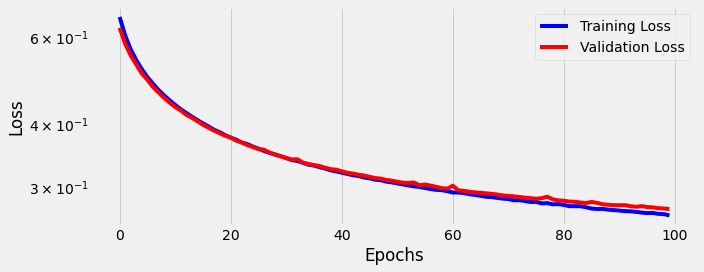
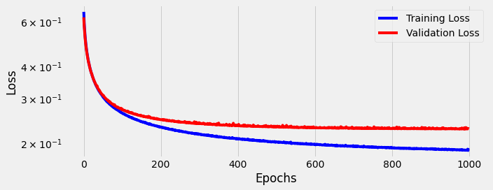
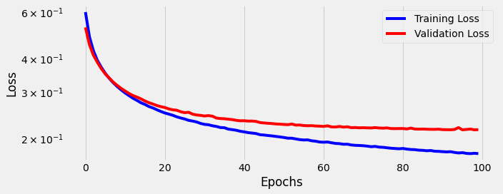
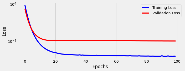
We train for 100 epochs using our training and validation data:
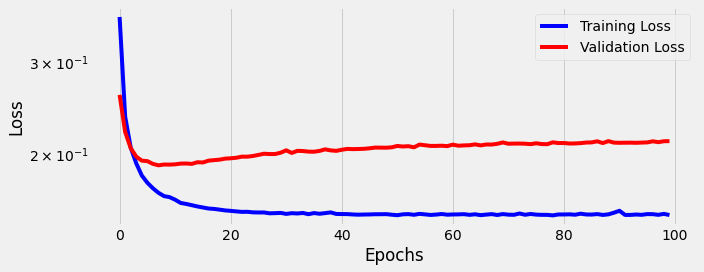
We see the model struggles to learn. As we proceed through 100 epochs the model overfits on the training data; the gap between training loss and validation loss becomes wide, and stays wide.
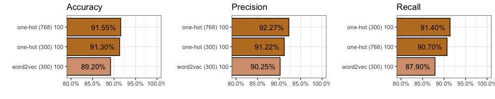
How well does the model do given One-Hot (300) encoding on data it has never seen before (our testing data, group 5)?
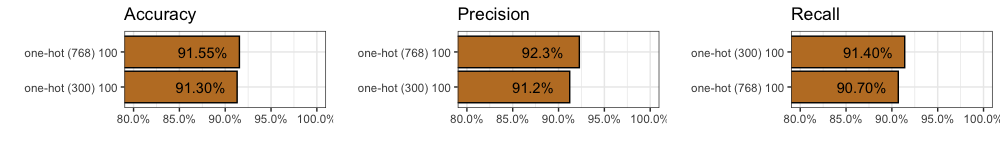
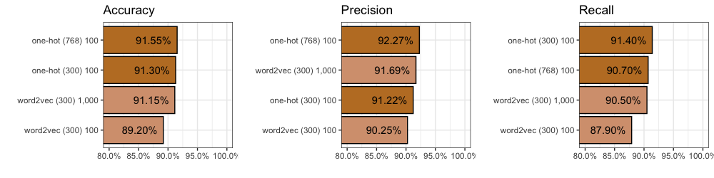
In terms of accuracy we got 91.3%. This means the model correctly classified 1,826 out of 2,000 comments. Not bad.
In terms of precision we got 91.2%. This means that of all the comments our model thought were from “Lord of the Rings”, 91.2% of them were actually from “Lord of the Rings”. It also means 8.8% were really from “Star Wars”.
In terms of recall we got 91.4%. This means that of the 1,000 “Lord of the Rings” comments in our training data (exactly half there are), our model found 914 of them.
You can find all 2,000 individual predictions on github.
One-Hot (768)
Can we make the model perform better by including more tokens? What if we use the top 768 tokens instead?
The data looks pretty much the same, except now we have another 468 columns of 0’s and 1’s. You can find the full data here on github. And you can train and test the model with python (google colab).
The only change to the model is more inputs. Now we have 769 total trainable parameters. We train for the same 100 epochs:
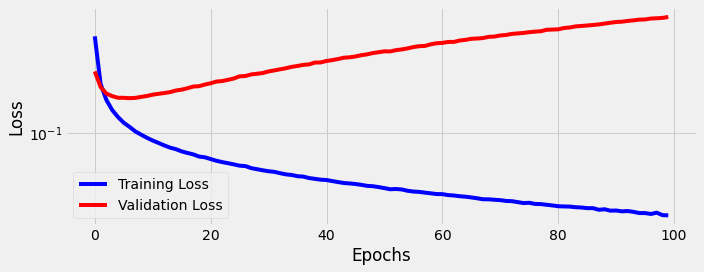
We see the model struggles to learn even more than before. The gap between training loss and validation loss gets wider as we train the model longer and longer.
We find accuracy improves (+0.35%) to 91.55%. We also find precision improves (+1.1%) to 92.3%, but recall decreases (0.7%) to 90.7%. You can find all 2,000 individual predictions on github if you’d like to take a closer look.
Obviously we can keep throwing more and more tokens at our model, but the law of diminishing returns is against us. Is there a better way to encode the information this text contains?
word2vec
Our approach to NLP encoding took a radical leap forward with the 2013 paper Efficient Estimation of Word Representations in Vector Space. Instead of representing each token with a simple 0 or 1, word2vec proposed representing each token as a vector instead.
![\[\vec{king} = \begin{bmatrix}0.125976562\\0.0297851562\\0.00860595703\\...\\0.251953125\end{bmatrix}\]](https://datajenius.com/wp-content/ql-cache/quicklatex.com-0c45bcfa747049fd96161bbfc0a9f2b3_l3.png "Rendered by QuickLaTeX.com")
We can use cosine similarity to compare how similar any two equal-length vectors are to each other:
![\[\text{CosSim}(\vec{a}, \vec{b}) = \frac{\vec{a} \cdot \vec{b}}{||\vec{a}|| \thinspace||\vec{b}||} = \frac{\sum_i^na_ib_i}{\sqrt{\sum_i^na_i^2}\sqrt{\sum_i^nb_i^2}}\]](https://datajenius.com/wp-content/ql-cache/quicklatex.com-d22cc3e8fb33f08e7c16c3fec94c8da5_l3.png "Rendered by QuickLaTeX.com")
This allows us find the tokens that are most similar to our given token (“king” in this example):
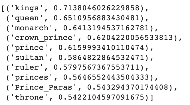
This also allows us to do the following:
![\[\vec{king}+\vec{woman}-\vec{man} = \text{???}\]](https://datajenius.com/wp-content/ql-cache/quicklatex.com-c4e5fb6d73dc2a6e639cb8111f226b87_l3.png "Rendered by QuickLaTeX.com")
Behind-the-scenes this is just vector addition and subtraction. We create a new vector:
![\[\begin{bmatrix}0.125976562\\0.0297851562\\0.00860595703\\...\\0.251953125\end{bmatrix} + \begin{bmatrix}0.243164062\\-0.0771484375\\-0.103027344\\...\\-0.0294189453\end{bmatrix} - \begin{bmatrix}0.32617188\\0.13085938\\0.03466797\\...\\0.02099609\end{bmatrix} = \begin{bmatrix}0.04296875\\-0.178222656\\-0.129089355\\...\\0.201538086\end{bmatrix}\]](https://datajenius.com/wp-content/ql-cache/quicklatex.com-2338b13252b5c22e0c18b7a11e87545a_l3.png "Rendered by QuickLaTeX.com")
We can then use cosine similarity to find which token in our existing vocabulary is most similar to this new hybrid vector:
![\[\vec{king}+\vec{woman}-\vec{man} = \vec{queen}\]](https://datajenius.com/wp-content/ql-cache/quicklatex.com-be9cfbf85ad410921bc4da42773dbf4c_l3.png "Rendered by QuickLaTeX.com")
These word2vec vectors are clearly more informative and flexible than our old One-Hot encoding. Can we use them to improve the performance of our model?
word2vec Tokenization
The original word2vec was trained on roughly 100 billion words from a collection of articles curated by Google News. It contains a vocabulary of 3 million unique tokens. We will tokenize on the same examples from above to see how it compares:
I love Luke Skywalker, but I hate Gandalf the Grey.
I love Gandalf the Grey, but I hate Luke Skywalker.
We find that word2vec’s vocabulary includes unigrams like our One-Hot encoding, but also and parts of words:
i love luke skywalker [UNK] but i hate ganda ##l ##f the gre ##y [UNK]
i love ganda ##l ##f the gre ##y [UNK] but i hate luke skywalker [UNK]
We see that word2vec’s vocabulary does not include punctuation; both the comma and period have been replaced with [UNK], which represents unknown tokens. We also see word2vec’s vocabulary does not include the name “Gandalf” and instead tokenizes it using two word fragments (“ganda” + “##l” + “##f”). These word fragment tokens allow word2vec to cover a much greater variety in language.
word2vec Word Embeddings
For each token in word2vec’s vocabulary, we have a 300-dimension word embedding, a vector with a series of 300 numbers.
![\[\vec{skywalker} = \begin{bmatrix}0.105957031\\0.04296875\\0.0810546875\\...\\0.171875\end{bmatrix}\]](https://datajenius.com/wp-content/ql-cache/quicklatex.com-9dc43a7ed32ad87b519b10773b618309_l3.png "Rendered by QuickLaTeX.com")
For special tokens (e.g. [UNK]) we simply use a vector of 300 zeros:
![\[\vec{[UNK]} = \begin{bmatrix}0\\0\\0\\...\\0\end{bmatrix}\]](https://datajenius.com/wp-content/ql-cache/quicklatex.com-755857c06580f14fbd0c2c6571b0ea95_l3.png "Rendered by QuickLaTeX.com")
Once we have tokenized our text, we simply grab the corresponding pre-trained word2vec word embedding for each of them. This includes our word fragment tokens like “##l” and “##f”.
word2vec Sentence Embeddings
We have 10,000 comments, each with a variable number of tokens, each of which is associated to a 300-dimension word embedding. How do we turn this mess into useable input for our model?
The first thing we will do is deal with the fact that our comments have variable numbers of tokens. We will set a max token length of 500, and truncate any comments that are longer than that. For comments shorter than 500 tokens, we will pad them with vectors of 300 zeros.
For example:
I love Gandalf the Grey, but I hate Luke Skywalker.
This is tokenized by word2vec like so:
i love ganda ##l ##f the gre ##y [UNK] but i hate luke skywalker [UNK]
And encoded like so:
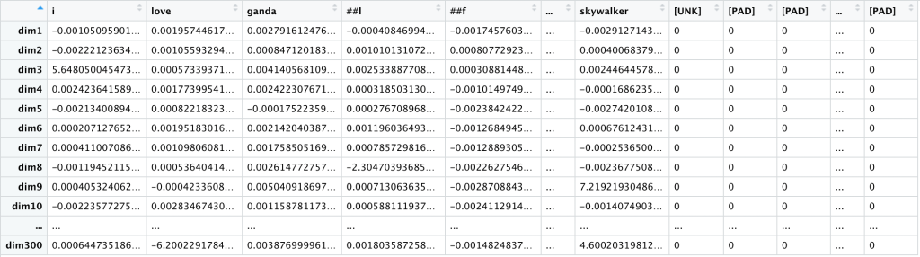
We now have exactly 500 columns left-to-right, one for each token in this comment, plus as many [PAD] tokens as needed. We also have exactly 300 rows, one for each of our 300 dimensions.
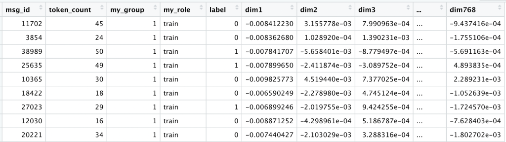
There are many different ways we might combine these token-based word embeddings into full sentence (comment) embeddings. One simple method is to take the average of each dimension, the row-wise mean of the above dataframe. If we take those averages and transpose them (rotate 90°) we get something that resembles our One-Hot encoding from above.
At this point our data for all comments looks like this:
Now we have one row for each comment, plus an additional 300 columns (our features X). However, instead of a simple 0 or 1 for a select vocabulary of tokens, we now have the average of each dimension of our 300-dimension word embeddings. What was once a sparse matrix full of 0’s is now dense with information.
Because these word2vec embeddings are pre-trained, we can encode all of our data at the same time without any fear of data leakage. You can find the full data here on github. And you can extract these embeddings yourself with python (google colab).
Limitations of word2vec
In theory, word2vec offers some advantages over One-Hot. For example, One-Hot ignores how often tokens are used. With word2vec, repeated tokens serve as a sort of weighted average in our sentence embeddings. We also noted that, in terms of One-Hot encoding, the tokens “love” and “loved” are completely different things. Not true of these word2vec embeddings:
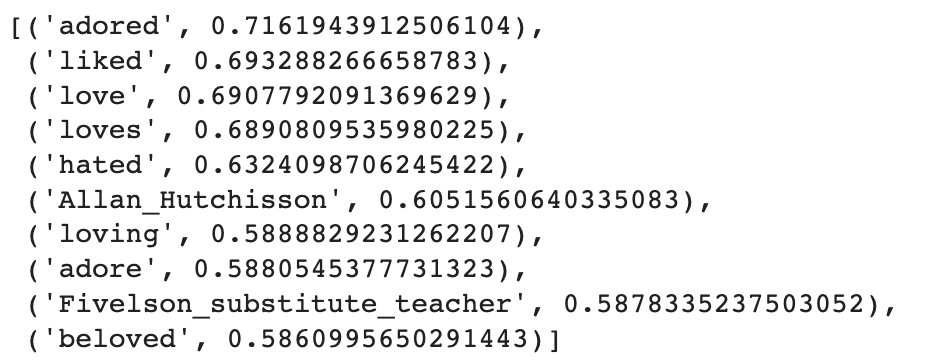
We see that the most similar tokens to “loved” not only include “love” but also “loves”, “loving”, “adore” and other synonyms and antonyms. This also shows how embeddings like these are able to deal with common slang, typos, and other eccentricities of natural language.
However, as with our One-Hot encoding, the order of tokens is still ignored. The “I love/hate Luke Skywalker, but I love/hate Gandalf the Grey.” examples still result in identical encodings. Furthermore, any tokens that do not appear in word2vec’s 3,000,000 token vocabulary will be encoded as zeros and lost.
And the biggest limitation to these word2vec embeddings? They were trained almost 10 years ago, on data not very similar to our Reddit comments. Consider the tokens most similar to “luke”:
It appears “luke” is associated to other common first names, nothing specific to our Jedi hero. And the tokens most similar to “skywalker”?
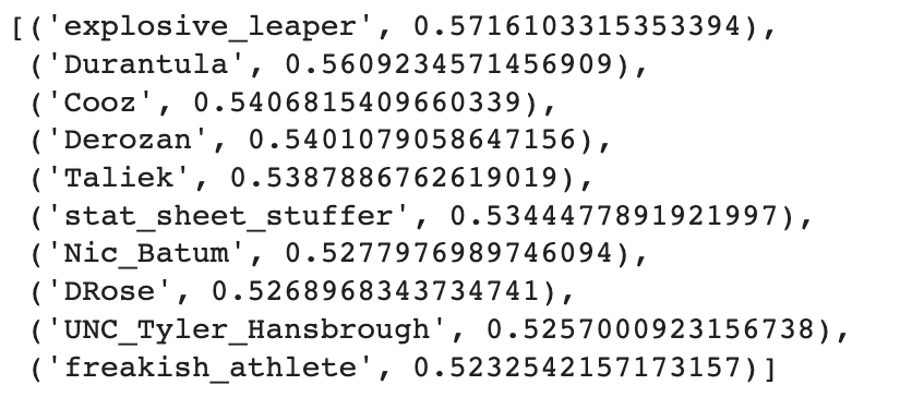
I’m not sure what these tokens have in common. Is this new word2vec encoding truly better than the old One-Hot 0’s and 1’s?
word2vec (300)
To train and use the model we turn back to python (google colab).
We will pass the model 300 inputs, the means of each of our 300 dimensions of word2vec embeddings for each comment. This results in 301 total trainable parameters (including the bias).

We train for 100 epochs using our training and validation data:
We see the model is now learning. The gap between training loss and validation loss is small, and both continue to decrease as the model trains longer and longer.
However, compared to our One-Hot inputs with 300 dimensions, after 100 epochs, we find accuracy decreases (-2.1%) to 89.2%. We also find precision drops (-0.97%) to 90.25%, and recall decreases (-2.8%) to 87.9%. You can find all 2,000 individual predictions on github if you’d like to take a closer look.
We continued training for 1,000 epochs:
Even after 1,000 epochs we found accuracy failed to beat our One-Hot inputs (-0.15%) with 91.15%. We find an improvement in precision (+0.47%) to 91.69%, but recall decreases (-0.2%) to 90.5%. You can find all 2,000 individual predictions on github.
Does this mean all these fancy vector encodings are a waste of time?
Custom Embeddings
The name “word2vec” usually refers to the pre-trained 300-dimensional word embeddings used above . However, “word2vec” can also refer the actual model used to train these embeddings in the first place. We aren’t stuck with these pre-trained vectors. We can build our own using the word2vec model and our own specific text.
Sure, we could just reuse the word2vec model, but what fun is that? In order to truly dig in and understand these embeddings, we are going to make our own, from scratch, using R.
The Theory
The theory behind word2vec is deceptively simple:
You shall know a word by the company it keeps.
John Rupert Firth
At the heart of any neural network we find a loss function, and word2vec is no exception:
![\[J(\theta) = -\frac{1}{T} \sum_{t=1}^T \sum_{j=(-m)}^m log\bigg(p(w_{t+j}|w_t;\theta)\bigg) \text{ where } j \neq 0\]](https://datajenius.com/wp-content/ql-cache/quicklatex.com-b176d69a7469dfd7e94f575f6297da0b_l3.png "Rendered by QuickLaTeX.com")
Although this formula appears intimidating at first, it can be reduced to some very simple ideas. (T) is the total number of tokens in our corpus. We loop through each of these tokens (t) one-by-one. At each token we look at a window of size (m) to see which tokens are our neighbors. To use an example, imagine the text:
Let us assume m=2 and t=5 for the sake of this example. This means we have reached the 5th token (“is”):
![\[\text{ machine } \text{ learning }\frac{\text{ is }}{} \text{ super } \text{ cool }\]](https://datajenius.com/wp-content/ql-cache/quicklatex.com-a7591c7aef2ef9f87e9f4e113e9778fe_l3.png "Rendered by QuickLaTeX.com")
Our m window of 2 means we look at the two words in front of “is”, and the two words that follow. Note that m=2 is an arbitrary choice, determined by the researcher.
One heuristic is that smaller window sizes (2-15) lead to embeddings where high similarity scores between two embeddings indicates that the words are interchangeable. […] Larger window sizes (15-50, or even more) lead to embeddings where similarity is more indicative of relatedness of the words.
Jay Alammar, The Illustrated Word2vec
Recall this term of our loss function:
![\[\sum_{j=(-m)}^m log\bigg(p(w_{t+j}|w_t;\theta)\bigg) \text{ where } j \neq 0\]](https://datajenius.com/wp-content/ql-cache/quicklatex.com-9730a451acfaa69a786d5afbbd624793_l3.png "Rendered by QuickLaTeX.com")
Here this simply means:
![\[log\bigg(p(\text{machine}|\text{is};\theta)\bigg) + log\bigg(p(\text{learning}|\text{is};\theta)\bigg) + log\bigg(p(\text{super}|\text{is};\theta)\bigg) + log\bigg(p(\text{cool}|\text{is};\theta)\bigg)\]](https://datajenius.com/wp-content/ql-cache/quicklatex.com-c4043e582ede7d4238b79a90eb4ae5de_l3.png "Rendered by QuickLaTeX.com")
It all comes down to basic probability. How likely is a context token given a specific target token?
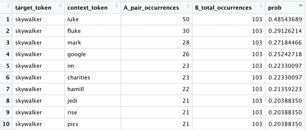
Let us simplify the above math. Let A equal the number of comments in which a target token appears together with a context token. Let B equal the number of comments in which the target token appears overall. Our probability is now a simple A/B.
Let us illustrate with an example:
![\[p(\text{luke}|\text{skywalker}) = \frac{A}{B} = \frac{50}{103} \approx 48.5\%\]](https://datajenius.com/wp-content/ql-cache/quicklatex.com-e95f89927304d9e0deba4462a0a6ee91_l3.png "Rendered by QuickLaTeX.com")
The token “skywalker” appears in 103 of our training comments. The tokens “skywalker” and “luke” appear together in 50 of our training comments. Therefore the probability of seeing the context token “luke” given the target token “skywalker” is roughly 50%.
Embeddings from Scratch
We can create custom embeddings with less than 200 lines of R code. Actually, we could do it more efficiently than that, but this code is intentionally verbose for the sake of a teaching example.
Because we are considering the entire comment regardless of length, our m window is now variable- the length of each individual comment. This results in the largest possible window, the largest possible m, and yields embeddings where similarity is more indicative of the relatedness of the words.
To avoid data leakage, we will build these custom embeddings based on our training data only:
############################################################
# load our TRAINING data from github (groups 1, 2, 3)
comments <- read.csv("https://raw.githubusercontent.com/DataJenius/NLPEncodingExperiment/main/data/comments/selected/selected_reddit_comments_group1.csv") %>%
  rbind(read.csv("https://raw.githubusercontent.com/DataJenius/NLPEncodingExperiment/main/data/comments/selected/selected_reddit_comments_group2.csv")) %>%
  rbind(read.csv("https://raw.githubusercontent.com/DataJenius/NLPEncodingExperiment/main/data/comments/selected/selected_reddit_comments_group3.csv"))
Again we tokenize into unigrams. B is simply the document frequency from before. We limit our vocabulary to tokens that have appeared in at least 2 comments:
############################################################
# define vocabulary that appears in at least 2 documents
# we have 10,161 unique tokens (our vocabulary)
vocab <- unigrams %>%
  group_by(token) %>%
  summarise(B_total_occurrences=length(unique(msg_id))) %>%
  arrange(desc(B_total_occurrences)) %>%
  filter(B_total_occurrences >= 2) %>%
  rename(target_token=token)
We can get A from the pairwise_count function: the number of times each context token appears with a given target token.
############################################################
# define all pairs of our 10,161 vocab words
vocab.pair <- unigrams %>%
  # only consider tokens in vocab
  filter(token %in% vocab$target_token) %>%
  # find A the occurrences of both tokens
  pairwise_count(token, msg_id, diag=FALSE) %>% # include diagonal (always 100%)
  rename(target_token=item1,
         context_token=item2,
         A_pair_occurrences=n)
We join the two together and calculate prob as A/B:
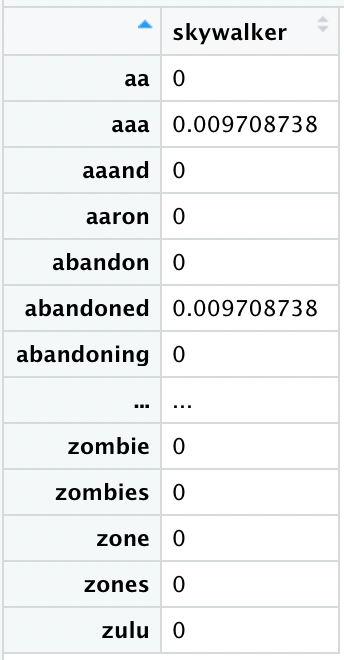
Next we cast this probability into a matrix where each row represents a target token and each column represents a context token. We have 10,161 rows and columns, one for each token in our vocabulary:
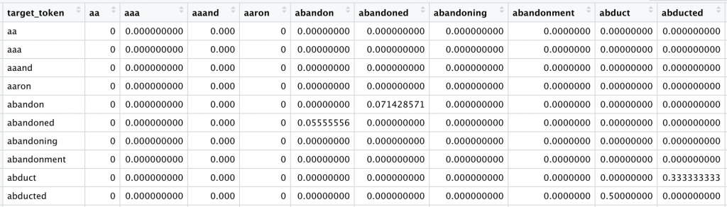
Once again we have a sparse matrix. If we take the row for a single target token and transpose it, what we are left with is a de-facto 10,161-dimension word embedding. Each dimension represents the probability of each of the 10,161 potential context tokens:
There are many different methods of dimensionality reduction we might use, including PCA, t-SNE and SVD, just to name a few. Here we will use IRLBA in order to reduce from 10,161 dimensions down to 300 dimensions, the same number our word2vec embeddings have:
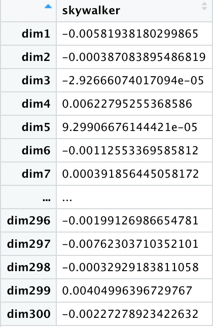
Our sparse matrix has become dense with information, but the trade-off is interpretability. We had 10,161 rows, each corresponding to a specific context token probability. Once reduced to 300, our dimensions no longer refer to a specific token. This makes it very hard to define what a given dimension is capturing in terms a human can understand.
We can, however, understand the essence of this new custom embedding: we have preserved the most important information contained in the above probability matrix.
Custom Sentence Embeddings
How do we use these new custom embeddings to encode our full comments? Our method will be similar to our word2vec sentence embeddings above, with one notable difference.
Instead of padding and truncating our comments to a standard number of tokens, we will simply consider all the tokens in each comment that can be found in our vocabulary. Any tokens not in our vocabulary will be ignored. Any comment without any known tokens will be encoded with 300 zeros instead.
Our custom vocabulary still includes 10,161 different unigrams. Each of these tokens is associated to one of the 300-dimension custom word embeddings we made above.
For example:
I love Luke Skywalker, but I hate Gandalf the Grey.
This is tokenized based on our custom vocabulary like so:
love luke skywalker hate gandalf grey
And encoded like so:
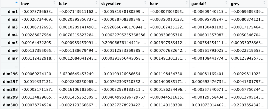
To reduce this into a sentence embedding, once again we will take the average per dimension (the row-wise mean) and transpose it. At this point our data for all comments looks like this:
You can find the full encoded data here on github. And you can encode this data for yourself using this R script.
Limitations of Custom
The order of tokens is still being ignored. The “I love/hate Luke Skywalker, but I love/hate Gandalf the Grey.” examples will still result in identical encodings. Furthermore, any tokens that do not appear in our custom 10,161 unigram vocabulary will be ignored.
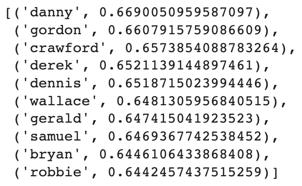
However, these custom embeddings seem to capture the essence of our comments far better than the pre-trained word2vec embeddings. Consider the most similar tokens for “luke” and “gandalf”:
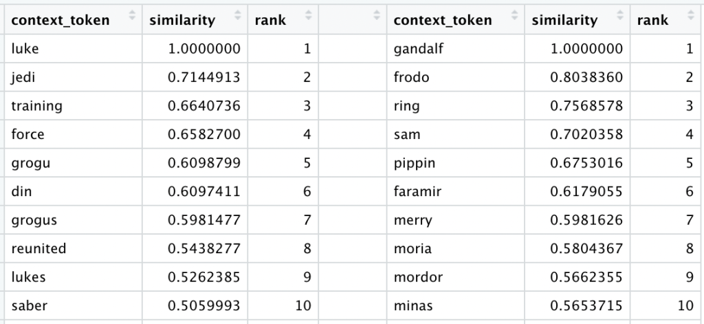
These similar tokens make a lot more sense now. Do we finally have an encoding that can beat the old One-Hot 0’s and 1’s?
Custom (300)
To train and use the model we turn back to python (google colab).
We will pass the model 300 inputs, the means of each of our 300 dimensions of custom embeddings for each comment. This results in 301 total trainable parameters (including the bias).

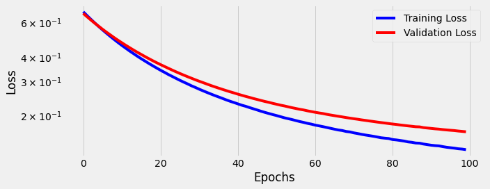
We train for 100 epochs using our training and validation data:
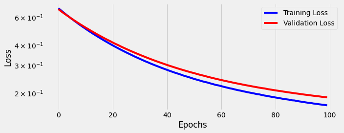
We see the model is learning. Both training loss and validation loss continue to decrease as the model trains longer and longer.
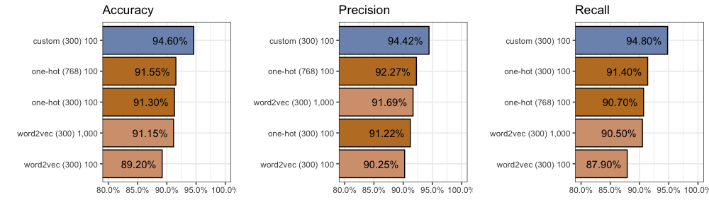
We find considerable improvement compared to our One-Hot inputs with 300 dimensions. After 100 epochs, accuracy increases (+3.3%) to 94.6%, precision increases (+3.2%) to 94.42%, and recall increases (+3.4%) to 94.8%.
You can find all 2,000 individual predictions on github.
We continued training for 1,000 epochs:
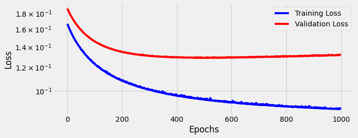
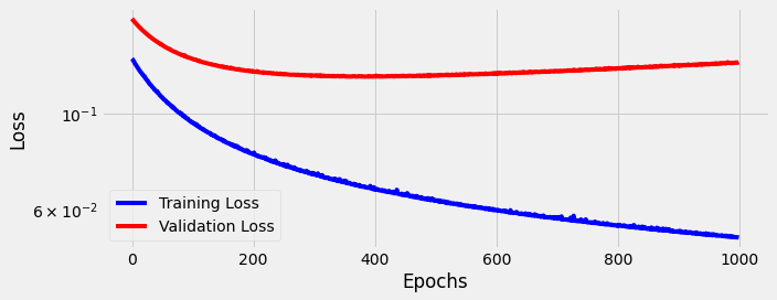
This training/validation loss curve isn’t as pretty now. After around 400 epochs it struggles to learn further, and starts to “unlearn” slightly as we approach 1,000 epochs.
Despite this, we see another jump in performance. Accuracy increases another +1.15% to 95.75%, while precision increases another +1.56% to 95.98%, and recall increases another +0.7% to 95.5%. Again you can find all 2,000 individual predictions on github.
It looks like our custom embeddings are pretty powerful.
Can we do better?
Custom (768)
What happens if we increase our custom embeddings to 768 dimensions?
The data looks pretty much the same, except now we have another 468 columns of dense custom embedding inputs. You can find the full data here on github. And you can train and test the model with python (google colab).

The only change to the model is more inputs. Now we have 769 total trainable parameters. We train for the same 100 epochs:
Once again we see the model is learning; training and validation loss decrease as the model trains longer and longer.
Given these additional dimensions, we find more improvement. Compared to our custom embeddings with 300 dimensions, after 100 epochs each, accuracy increases (+0.75%) to 95.35%, precision increases (+0.98%) to 95.4%, and recall increases (+0.5%) to 94.8%. You can find all 2,000 individual predictions on github.
We continued training for 1,000 epochs:
Again the model starts to “unlearn” around the 400th epoch. Performance remains largely unchanged. We are unable to beat 300 dimensions with 768 dimensions after 1,000 epochs.
We could keep adding dimensions and training epochs, but once again we are facing the law of diminishing returns. If we want to improve performance further, we will need a different strategy.
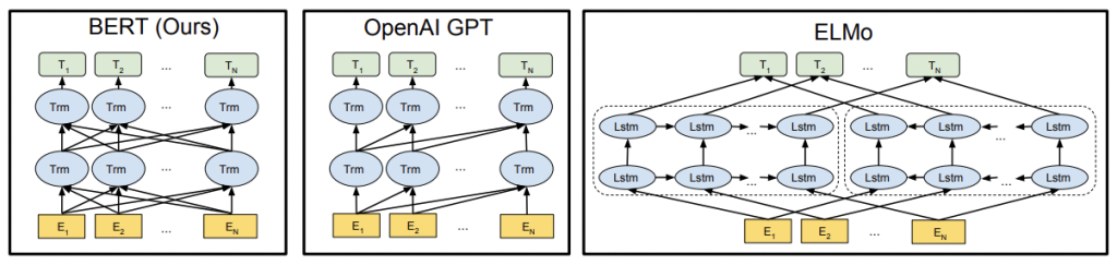
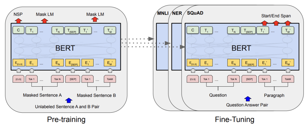
BERT
BERT (Bidirectional Encoder Representations from Transformers) combined the unsupervised pre-training of a transformer (OpenAI GPT) with embeddings that consider the bidirectional context of tokens (eLMo). When released in 2019, BERT was capable of producing state-of-the-art results for 11 different NLP tasks. Here we are concerned with only one of those tasks: classification.
Language Understanding
BERT Masking
One of the things BERT does is use masks in order to predict a token given the context of surrounding tokens. For example:
I [MASK] Luke Skywalker, but I hate Gandalf the Grey.
How does this differ from word2vec?
Until now, all of our encoding schemes have ignored the order of our tokens. A word2vec embedding trained with a window of m=9 would include “love”, “hate”, “Luke Skywalker” and “Gandalf the Grey”, but have no additional context beyond that.
By comparison, BERT is bidirectional. In other words, not only does BERT consider the order of tokens, it considers them both left-to-right and right-to-left.
I
I
At long last, the “I love/hate Luke Skywalker, but I love/hate Gandalf the Grey.” examples will result in different encodings, based on the specific order of the tokens.
BERT Tokenization
Let’s take a closer look at the BERT tokenizer:
I love Gandalf the Grey, but I hate Luke Skywalker.
This is tokenized by BERT like so:
[CLS] i love gan ##dal ##f the grey , but i hate luke sky ##walker . [SEP]
The first thing we notice about BERT tokenization is the special [CLS] token added to the start of our comment. This is going to be critical in the next step. We also find [SEP] tokens at the end of our comments. Unlike word2vec, BERT tokenization includes punctuation. Our comma and period remain.
We find that text tokenized by BERT, like word2vec, includes parts of words. However, unlike word2vec, BERT uses the WordPiece algorithm in order to define these subword tokens.
Intuitively, WordPiece is slightly different to BPE in that it evaluates what it loses by merging two symbols to ensure it’s worth it.
HuggingFace Documentation
BERT has a vocabulary of only 30,522 unique tokens, compared to word2vec’s vocabulary of 3 million. Despite this, we find that the BERT tokenizer with WordPiece is more versatile. It can handle pretty much whatever you throw at it:
Captain Smurgleblorp snorged his 😜 on Blursday.
[CLS] captain sm ##urg ##le ##bl ##or ##p s ##nor ##ged his [UNK] on blur ##sd ##ay . [SEP]
As before, when it encounters something unknown (in this case our 😜 emoji) you will see the special [UNK] token in its place.
These tokens look good. But how do we get our embeddings?
BERT Sentence Embeddings
For our word2vec and custom sentence embeddings above, our process was roughly the same:
- Tokenize our text and extract all known tokens
- Encode each known token with the corresponding word embedding
- Use the dimension-wise average as the sentence embedding
BERT, like word2vec above, uses truncation and padding to turn comments (each with a variable number of tokens) into a standard size tensor. However, this is where the similarities end.
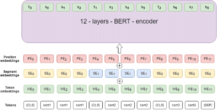
BERT uses 12 transformer layers and 12 self-attention heads in order to focus on different sections of each text (reading both left-to-right and right-to-left). The resulting embeddings are based (in part) on the order of tokens, and the exact position of the token in question. This is how BERT is able to train and learn 768-dimension contextual embeddings for each token.
This includes the special [CLS] token mentioned above.
We will use this special [CLS] embedding, rather than a dimensional average, for our downstream task (predicting which franchise a comment belongs to). As we see below, this is exactly what the BertForSequenceClassification model does:
BertForSequenceClassification(
  (bert): BertModel(
    (embeddings): BertEmbeddings(
      (word_embeddings): Embedding(30522, 768, padding_idx=0)
      (position_embeddings): Embedding(512, 768)
      (token_type_embeddings): Embedding(2, 768)
      (LayerNorm): LayerNorm((768,), eps=1e-12, elementwise_affine=True)
      (dropout): Dropout(p=0.1, inplace=False)
    )
    (encoder): BertEncoder(
    	** 12 layers of self-attention goodness **
    )
    (pooler): BertPooler(
      (dense): Linear(in_features=768, out_features=768, bias=True)
      (activation): Tanh()
    )
  )
  (dropout): Dropout(p=0.1, inplace=False)
  (classifier): Linear(in_features=768, out_features=2, bias=True)
)
We used this python script (google colab) to extract the output of the BertPooler above. Note that we used the pre-trained (pt) “bert-based-uncased” model to get these. Like the our word2vec input above, this BERTpt input is not based on any of our own comment data. These embeddings are based on what BERT saw back in 2019 when it was originally trained.
bert_model = TFBertModel.from_pretrained(
    'bert-base-uncased',
    trainable=False,
    num_labels=2)
At this point our data is almost identical to custom (768), just with different values for each dimension. It looks like this:
You can find the full encoded data here on github.
BERTpt (768)
To train and use the model we turn back to python (google colab).
We will pass the model 768 inputs, the pre-trained BERT [CLS] embeddings for each comment. This results in 769 total trainable parameters (including the bias).

Because the values of these BERTpt embeddings are significantly larger that the others, we reduced our initial learning rate (η) to 0.0003 to compensate. Then we train for 100 epochs using our training and validation data:
We see that our same simple classification model is able to learn from these fancy BERT embeddings too. Both training loss and validation loss decrease as the model trains.
How well do these new BERTpt embeddings do as input?
In a word: disappointing. The BERTpt input fails to outperform the one-hot or word2vec inputs. Custom still reigns supreme. You can find all 2,000 individual predictions on github.
Does this mean using BERT is a waste of our time? Not so fast.
Fine-tuning BERT
As mentioned above, BERT uses 12 transformers and 12 self-attention heads in order to generate these embeddings. However, the above pre-trained encoding didn’t take full advantage of that.
The excellent Illustrated BERT, ELMo, and co. (How NLP Cracked Transfer Learning) by Jay Alammar can help provide readers with some additional context. For our purposes the key point is this: we can fine-tune BERT.
Language Understanding
Unlike prior attempts at transfer learning, BERT allows us to fine-tune using all 109,483,778 of its trainable parameters. This results in the best possible representations of our specific text.
Once again we remain mindful of data leakage. We restrict this tuning to our training and validation data only, and keep our test data unseen. We used this python script (google colab) to fine-tune BERT for a single epoch. We then extracted these fine-tuned (BERTft) embeddings for all 10,000 comments for use in our own model.
While extracting these embeddings you will encounter the biggest limitation of BERT. Compared to our simple model, which trains and predicts in under five minutes, BERT can feel painfully slow. It took roughly 4 hours to complete a single epoch of fine-tuning. Why so long? Because we are fine-tuning 109,483,778 trainable parameters. That’s a lot of math.
Our end result is almost identical to custom (768) and BERTpt (768). All that changes is the specific values for each dimension.
It looks like this:
You can find the full encoded data here on github.
BERTft (768)
To train and use the model we turn back to python (google colab).
We will pass the model 768 inputs, the fine-tuned BERT [CLS] embeddings for each comment. This results in 769 total trainable parameters (including the bias).
We reduce our initial learning rate (η) to 0.00001 and train for 100 epochs using our training and validation data:
Both training loss and validation loss decrease as the model trains, but learning seems to level off after around 18 epochs.
Now the million dollar question: how do fine-tuned BERT embeddings compare to our best custom embeddings? We find accuracy improves (+0.65%) to 96.4%, precision improves (+0.61%) to 96.59%, and recall increases (+0.7%) to 96.2%.
You can find all 2,000 individual predictions on github if you’d like to take a closer look.
Eat your heart out, custom. It looks like BERT is the new sheriff in town.
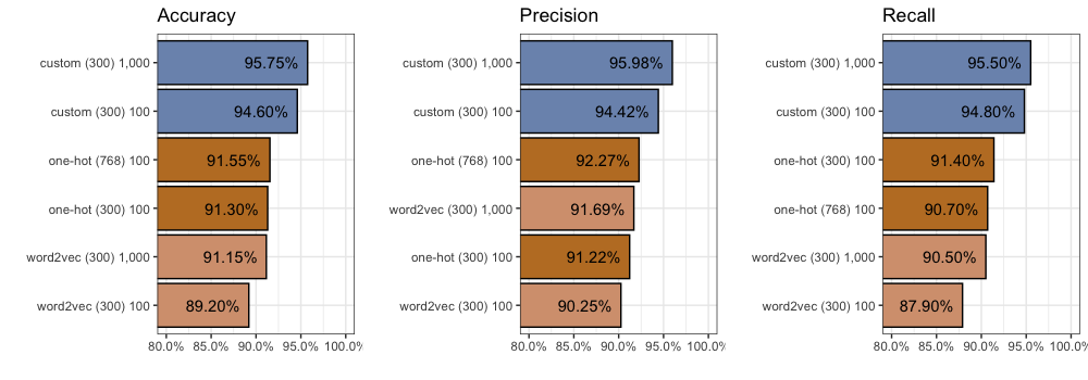
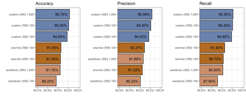
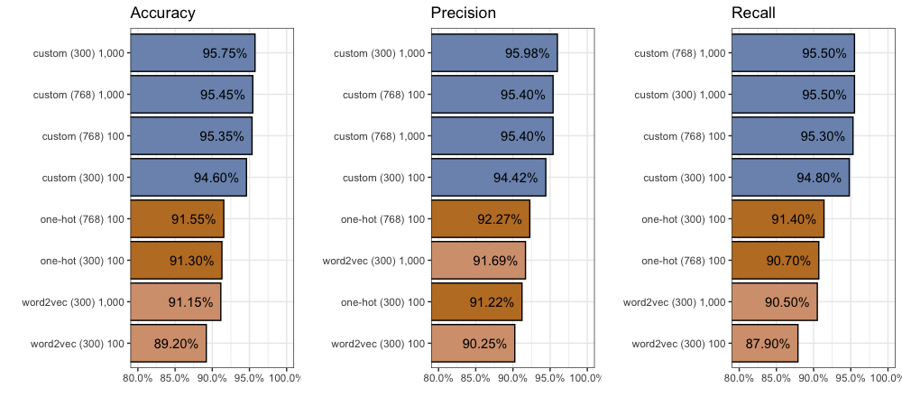
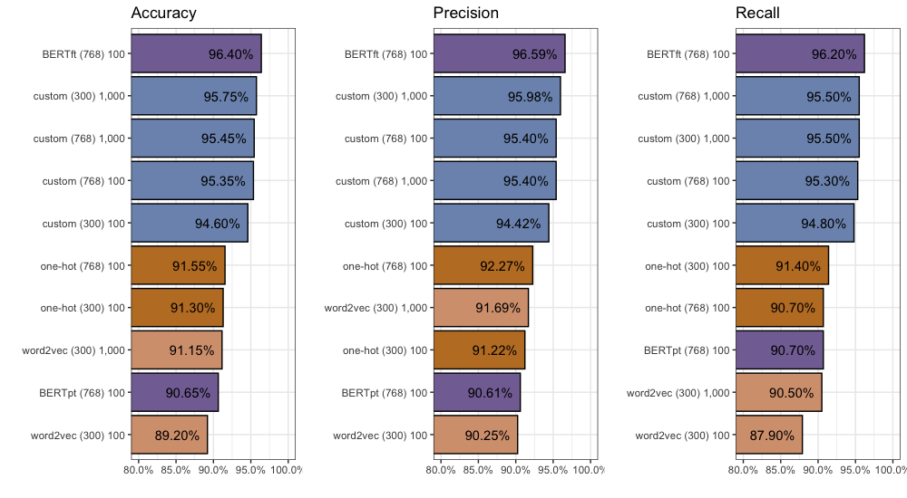
Comparing our Methods
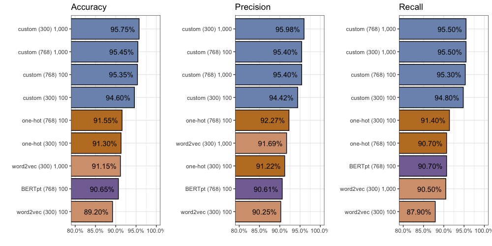
Here is a quick recap of the 10 different methods we have tried:
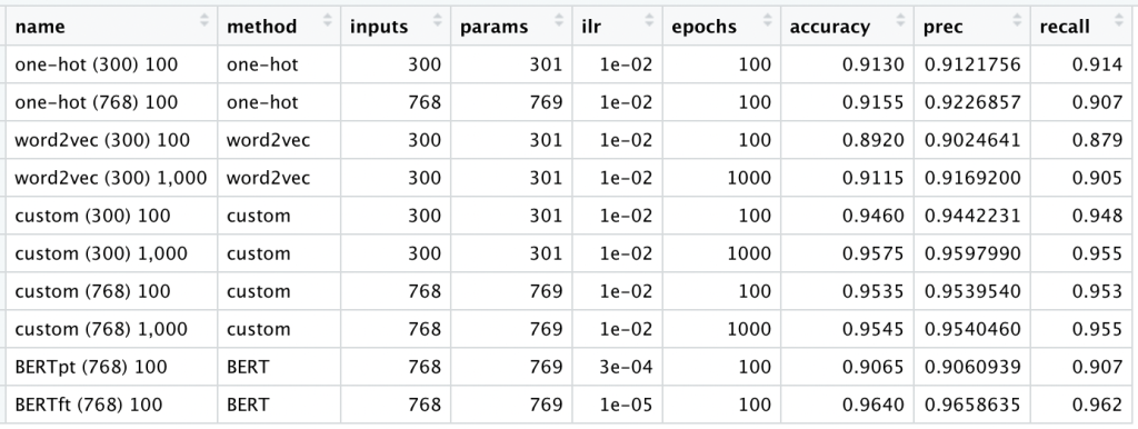
Beyond these statistics, we can gain some more intuition towards these different input methods by looking at some specific examples.
Easy Examples
Recall that our model predictions include the probability of belonging to the positive class (“Lord of the Rings”). This means we can look beyond accuracy, precision and recall, and see how confident the model was for each answer.
Consider this comment (from “Star Wars”):
“For over a thousand generations the Jedi knights were the guardians of peace and justice in the old republic. Before the dark times. Before the empire.”- Ben Kenobi to Luke Skywalker.
This is how each method responded:
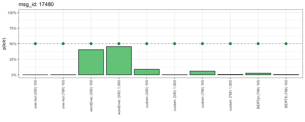
Our decision boundary is 50% (the dotted line). Everything over that line is classified as “Lord of the Rings”. Because this example comes from “Star Wars”, here we want all of these probabilities to be as low as possible. The closer a method is to 0%, the more confident it is that this is a “Star Wars” comment.
We can see that although our word2vec methods got this one right, they were the least right of the 10 methods tested. Compare to One-Hot and BERT which are much closer to 0%.
Consider this comment (from “Lord of the Rings”):
Start with The Hobbit:
1. Watching The Hobbit first doesn’t really spoil anything in The Lord of the Rings, whereas watching The Lord of the Rings first does spoil major plot elements in The Hobbit.
2. The Hobbit is shorter and you can start with the extended editions: those extra 12 minutes in the first film aren’t going to make or break anyone’s viewing experience.
This is how each method responded:
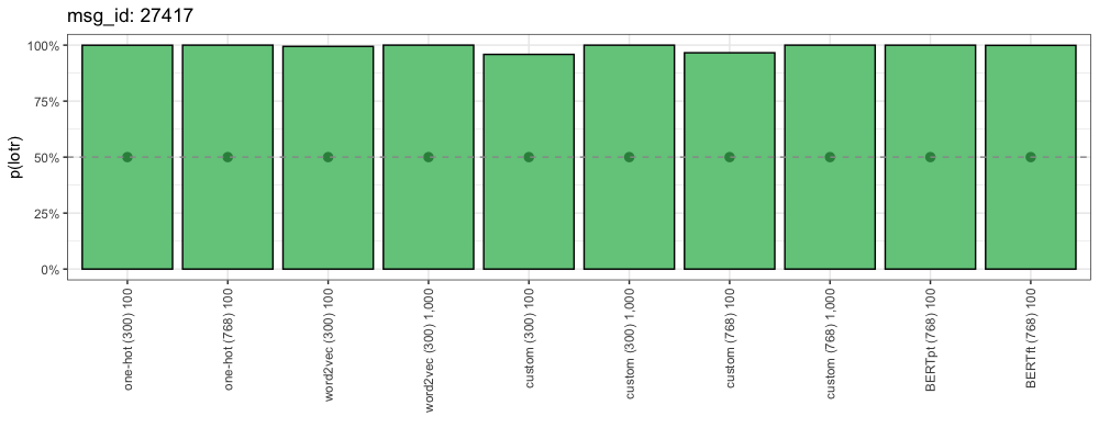
Because this comment is from our positive class (“Lord of the Rings”) here we want to see all of these probabilities as high as possible. The closer a method is to 100%, the more confident it is that this is a “Lord of the Rings” comment.
These comments are both rich with franchise-specific terms like “Jedi”, “Ben Kenobi”, “Luke Skywalker”, “Hobbit” and even “The Lord of the Rings”. We can understand why all methods got these right- these were some easy ones.
Not As Easy Examples
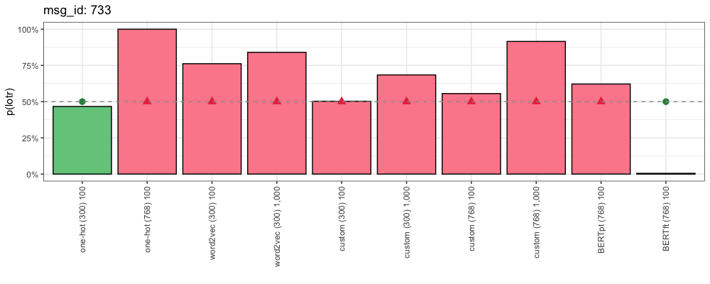
Consider this comment (from “Lord of the Rings”):
I’m halfway through the Two Towers right now (third reading). I hope you make it!
Props for trying at 11. I tried it when I was in grade 2. I don’t remember if I made it through, but I once found copies of the Ent’s songs in and old journal from that time haha
This is how each method responded:
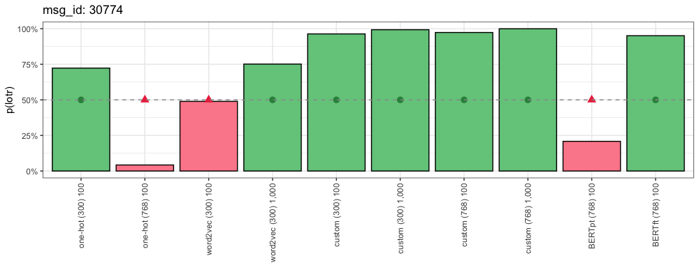
We humans recognize “Two Towers” as the title of one of the “Lord of the Rings” books. Why did our One-Hot encodings struggle here? Because the critical token “towers” does not appear in the vocabularies of One-Hot (300) or One-Hot (768). And the pre-trained word2vec and BERT embeddings don’t recognize the significance of “Two Towers” here.
Compare to our custom (300) embeddings:
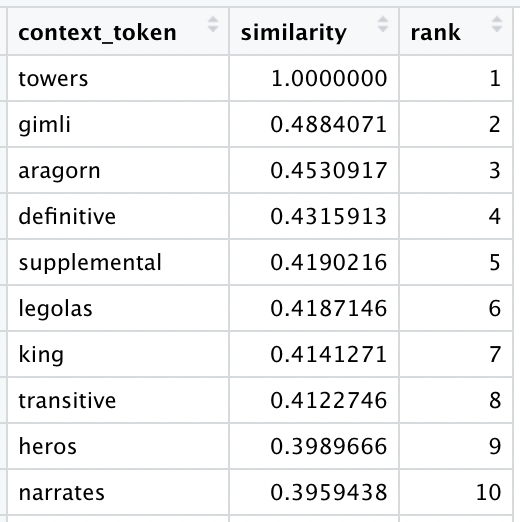
Not only does our custom vocabulary include “towers”, it associates that token to “gimli”, “aragorn” and “legolas”. Presumably our fine-tuned BERT embeddings were able to find a similar pattern, and come to a similar conclusion.
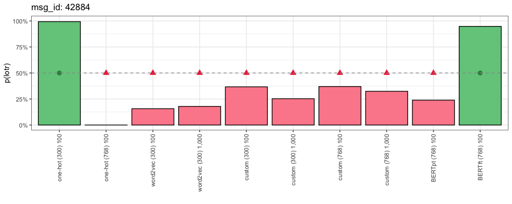
Our next comment (from “Star Wars”) dares to discuss the important issues: Does “Jabba the Hutt” reproduce asexually?
Yes it literally does. Asexual reproduction. That user isn’t talking about the Hutt’s sexual orientation, they’re talking about how they reproduce. But if they reproduced asexually, they would not have males and females
This is how each method responded:
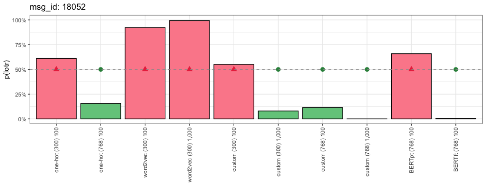
Similar to above, the critical token “hutts” does not appear in the vocabularies of One-Hot (300) or One-Hot (768). Likewise, the pre-trained word2vec and BERT embeddings don’t recognize this as a character from “Star Wars”. Even our custom (300) and custom (768) embeddings disagree here.
Let’s take a closer look at the most similar tokens to “hutts” according to both custom (300) and custom (768):
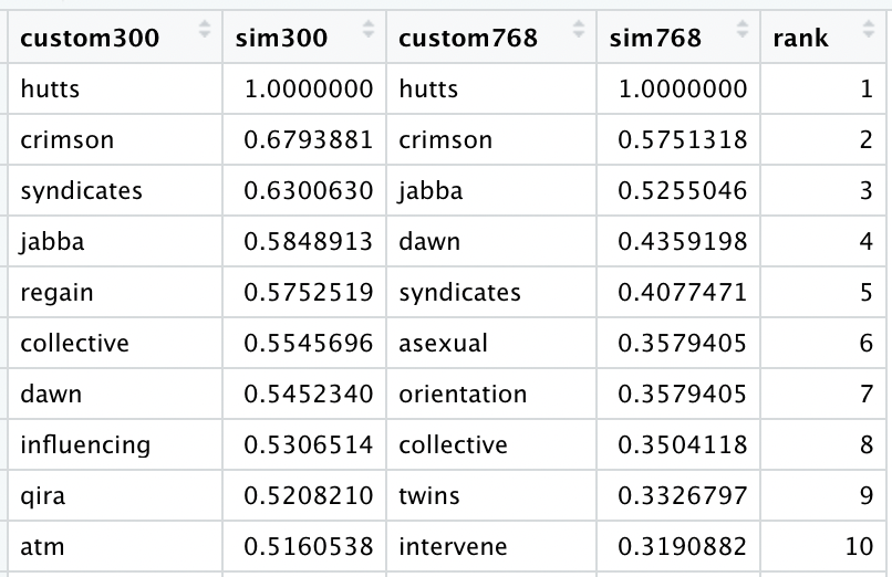
Both embeddings associate back to “jabba”, but only custom (768) contains enough dimensionality to also associate with “asexual” and “orientation”. Note that both custom embeddings (300 and 768) include the same 10,161 token vocabulary.
It takes custom (300) 1,000 epochs to get it right. With the added dimensionality, custom (768) figures it out after only 100.
Where BERT Prevails
Consider this comment (from “Star Wars”):
Their subscriber base surely expanded due to Mando and its great word of mouth. If BoBF were as good as Mando and built similar goodwill, it would expand their subscriber base even more. BoBF’s bad rep might not have shrunk it much, but they lost out on all the new subscribers they could have gained. Sure, there are diminishing returns after each additional good show, but they’d still be getting more money than they would by producing crap, and it’s not like slightly better writing would have added much in production costs.
This is how each method responded:
This comment uses slang (“Mando”, “BoBF”) to refer to the shows “The Mandalorian” and “The Book of Boba Fett”. The token “mando” appears in all of our One-Hot and custom vocabularies. “bobf” appears in our custom and One-Hot (768) vocabularies. Despite this, only our fine-tuned BERT embeddings resulted in a confident right answer.
Consider this comment (from “Lord of the Rings”):
Thinking about it now, I wonder if it was because they had some crumb of power because suddenly the world was giving them attention.
And it just went to their heads. They needed to flex that they should be considered as an absolute authority.
Makes me think of an old boss. Couldn’t handle a woman who said no. He grew up being rejected by them, but now that he was a manager, he just lost his shit whenever his control was threatened.
I think it was the same thing. Finally they were an expert at something, and they just had to show everyone in the most awkward way possible.
Most people just say “The book was better”, like that’s some sort of secret surprise to anyone.
That’s a given. With everything. Since ever. But they just need to let everyone know they read the book.
This is how each method responded:
Here is an interesting case where only our most simple encoding (One-Hot with top 300 tokens) and our most complicated encoding (fine-tuned BERT) got the right answer. And they are both pretty confident about it. What is going on here?
Out of our 298 training examples that included the token “book”, 70.5% of them came from “Lord of the Rings”.
Our One-Hot (300) encoding focuses on “book” because (a) it only looks for 300 tokens in the first place, and (b) this is the most relevant token in this example.
Our fine-tuned BERT encoding also focuses on the token “book”, despite having more than 100 million additional trainable parameters. This is the power of self-attention, and a good example of how BERT learns which parts of a text are the most relevant.
Given the length of this comment, our other encoding methods get overwhelmed with too much information. Once we look for 768 One-Hot encoded tokens, or take the dimension-wise averages of all the tokens this comment contains, our encodings lose their focus on “book”, and confuse the model.
Sentence Similarity
When looking at our word embeddings above, we used cosine similarity to rank how close tokens are to each other.
Can we use this same function to see how similar our sentence embeddings are to each other? Yes we can.
Custom Similarity
Consider the following comment (from “Lord of the Rings”):
If I am correct, Sam notes Gandalf’s true power when he effortlessly lifts I can’t remember what. But the frail old man is acf even as Gandalf the Grey.
If we compare the cosine similarities of our custom (768) sentence embeddings, we find this is the most similar comment:
Is it actually lore that their power is restrained? As in externally. I thought that they chose not use their power, though a portion of gandalf’s true power does slip through a couple of times. I think Sam notes his strength when he lifts frodo up to Glorfindel’s horse.
Edit: it was in Moria after Frodo got stabbed by the troll. Gandalf wasn’t present when Glorfindel picked him up after weathertop.
For the sake of comparison, here is another comment which also contains the name “Gandalf”, but has a much lower similarity score:
gandalf better not appear in this, that makes no sense, but I like the lotr universe becuase its set themed to the somewhat forgotten ancient culture of the British Isles.
This comment mentions “Gandalf”, but not his true power. We can see how this is less similar to the original comment.
BERT Contextual Embeddings
Consider the following examples:
In these examples, “feet” refers to a measurement of 12 inches.
In these examples, “feet” refers to the things attached to the bottom of your legs. This is a common phenomenon in natural language: the same words can have different meanings, depending on their context.
Let us compare to this example:
When we convert these into pre-trained BERT embeddings and compare cosine similarity, we see something amazing:
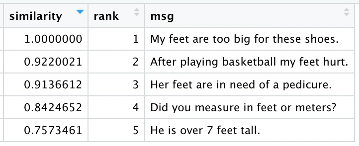
The BERT embeddings for “feet” (with toes) are more similar than the embeddings for “feet” (12 inches). The 12 transformers and self-attention heads of BERT are powerful enough to produce more informative embeddings.
Consider the following:
In these examples, “park” refers to the act of putting a vehicle to rest.
In these examples, “park” refers to a place you might want to go.
Let us compare to this example:
Again we convert these into pre-trained BERT embeddings and compare cosine similarity, and again we see something amazing:
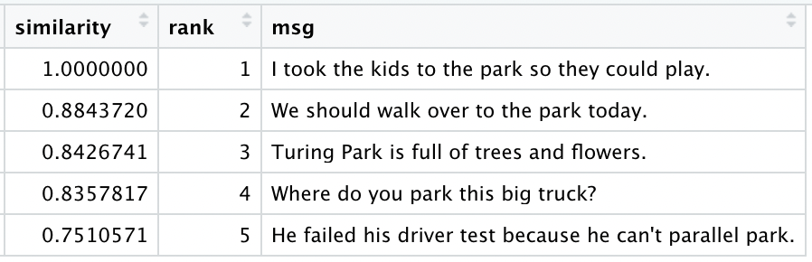
The BERT embeddings for “park” (noun) are more similar than the embeddings for “park” (verb). Once again BERT demonstrates the power of context in understanding natural language.
Conclusion
Back in the ancient times, before 2013, we usually encoded basic unigram tokens using simple 1’s and 0’s in a process called One-Hot encoding. word2vec improved things by expanding these 1’s and 0’s into full vectors (aka word embeddings). BERT improved things further by using transformers and self-attention heads to create full contextual sentence embeddings.
Beyond use in this classification example, these embeddings are powerful. They allow us to do math with words:
These embeddings also allow us to find the meaning of specific tokens, and compare the similarity of full sentences (comments). We can use BERT embeddings for many other tasks too, such as extracting a questions/answers model, or summarizing key points of text. This article has only scratched the surface in regards to BERT’s full capabilities.
When training models, it is often tempting to toss more features at it, train for more epochs, and hope for the best. This article demonstrates the diminishing returns such an approach will yield.
Instead we must think deeply about the information our text contains, and how we can represent that information numerically. As the above experiment proved, how we choose to encode our data can make all the difference.
Want more content like this? Please subscribe and share below: